Binary orbit
[1]:
import matplotlib.pyplot as plt
import numpy as np
[2]:
from exogaia.data import EpochAstrometry
from exogaia.leastsq import LeastSquares
from exogaia.models import KeplerModel
from exogaia.results import SamplingResults
from exogaia.samplers import MCMCSampler, NestedSampler
In preparation for Gaia DR4, the Gaia archive is in evolution. Unfortunately, it may be unstable at times and particular types of queries may time out. Please consider registering for a user account (https://www.cosmos.esa.int/web/gaia-users/register). For questions or advice, please contact the Gaia helpdesk (https://www.cosmos.esa.int/web/gaia/gaia-helpdesk).
[3]:
np.random.seed(42)
Gaia epoch astrometry
The EpochAstrometry class is used for storing Gaia epoch astrometry. For now, we can simulate epoch astrometry for Gaia DR4 or DR5. To do so, we can either set the stellar parameters manually or retrieve parameters from DR3.
In this example, we simulate a binary system by manually providing the stellar parameters. We choose a relatively small orbit such that most of the phase is well sampled by the simulated measurements.
[4]:
primary_mass = (1.0, 0.1)  # (Msun)
mass_2 = 0.01  # (Msun)
flux_ratio = 0.0
[5]:
epoch_astrom = EpochAstrometry(primary_mass=primary_mass, gaia_release='DR4')
----------------
Epoch astrometry
----------------

Gaia release: DR4
Reference epoch: 2017.5

Primary mass (Msun): 1.00 +/- 0.10
[6]:
model_param = {
    'ra': 50.0,
    'dec': 20.0,
    'parallax': 10.0,
    'pm_ra': -30.0,
    'pm_dec': 30.0,
    'g_mag': 7.0,
    'ecc': 0.3,
    'tau': 0.5,
    'inc': np.radians(60.),
    'aop': np.radians(4.),
    'pan': np.radians(90.),
    'sma': 2.,
}
[7]:
model_param = epoch_astrom.simulate_data(
    model_param=model_param,
    mass_2=mass_2,
    flux_ratio=flux_ratio,
    occ_rate=None,
    sigma_per_ccd=None,
    csv_out=None,
)
-------------
Simulate data
-------------

System type: binary

Primary mass (Msun): 1.00 +/- 0.10

AL scan uncertainty (per CCD) = 159.98 uas
AL scan uncertainty (per transit) = 56.56 uas

Additional parameters:
   - Primary mass (Msun) = 1.00
   - Companion mass (Msun) = 1.00e-02
   - Mass ratio = 1.00e-02
   - Flux ratio = 0.00e+00
   - Relative semi-major axis (au) = 2.00

-----------------------
Calculate stellar track
-----------------------

Stellar parameters:
   - RA offset (mas) = 0.000
   - Dec offset (mas) = 0.000
   - Parallax (mas) = 10.000
   - Proper motion in RA (mas/yr) = -30.000
   - Proper motion in Dec (mas/yr) = 30.000

---------------------
Calculate orbit model
---------------------

Orbit parameters:
   - Period (days) = 1027.956
   - Eccentricity = 0.300
   - Relative time of periastron = 0.500
   - Semi-major axis (mas) = 20.000
   - Inclination (deg) = 60.000
   - Argument of periastron (deg) = 4.000
   - PA of ascending node (deg) = 90.000

Applying AL bias from binarity:
   - Unresolved epochs = 36 / 70
   - Marginally resolved epochs = 34 / 70
   - Resolved epochs = 0 / 70
Infer parameters with least-squares
[8]:
leastsq = LeastSquares(epoch_astrometry=epoch_astrom)
[9]:
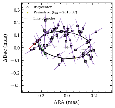
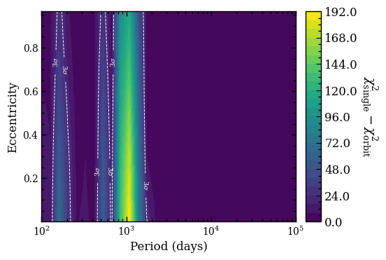
fig = leastsq.orbit_grid(map_type='chi2_det', n_sigma=[3], plot_file='plot.png', n_points=30)
--------------------------
Orbit grid (12-parameters)
--------------------------
Best-fit RUWE = 0.994

Best-fit stellar track:
   - RA offset (mas) = -0.018 +/- 0.018
   - Dec offset (mas) = -0.014 +/- 0.012
   - Parallax (mas) = 10.021 +/- 0.014
   - mu in RA (mas/yr) = -30.000 +/- 0.009
   - mu in Dec (mas/yr) = 29.999 +/- 0.006

Best-fit orbit:
   - Period (days) = 1082.637
   - Eccentricity = 0.400
   - Relative time of periastron = 0.43
   - Thiele-Innes A = -0.005 +/- 0.013
   - Thiele-Innes B = -0.191 +/- 0.020
   - Thiele-Innes F = 0.121 +/- 0.016
   - Thiele-Innes G = -0.075 +/- 0.020

Derived parameters:
   - Semi-major axis of photocenter (mas) = 0.211 +/- 0.019
   - Relative semi-major axis (au) = 2.070
   - Mass function (Msun) = 1.056e-06
   - Companion mass (Msun) = 1.025e-02

Conversion to campbell elements:
   - Period = 1082.637 days
   - Eccentricity = 0.400
   - Relative time of periastron = 0.433
   - Semi-major axis of photocenter (mas) = 0.211
   - Inclination (deg) = 58.087
   - Argument of periastron (deg) = 150.460
   - PA of ascending node (deg) = 105.186
[10]:
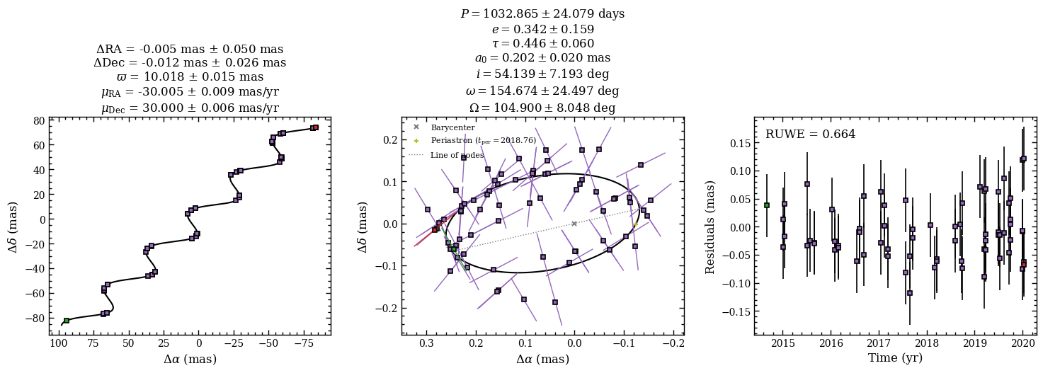
fig = leastsq.orbit_fit(inc_jitter=False, plot_file='plot.png')
-------------------------
Orbit fit (12 parameters)
-------------------------

Reduced chi^2: 0.441
RUWE: 0.664

Best-fit stellar track:
   - RA offset (mas) = -0.005 +/- 0.050
   - Dec offset (mas) = -0.012 +/- 0.026
   - Parallax (mas) = 10.018 +/- 0.015
   - mu in RA (mas/yr) = -30.005 +/- 0.009
   - mu in Dec (mas/yr) = 30.000 +/- 0.006

Best-fit orbit:
   - Period (days) = 1032.865 +/- 24.079
   - Eccentricity = 0.342 +/- 0.159
   - Relative time of periastron = 0.446 +/- 0.060
   - Semi-major axis of photocenter (mas) = 0.202 +/- 0.020
   - Inclination (deg) = 54.139 +/- 7.193
   - Argument of periastron (deg) = 154.674 +/- 24.497
   - PA of ascending node (deg) = 104.900 +/- 8.048

Number of function evaluations: 10
Number of Jacobian evaluations: 10

Derived parameters:
   - Relative semi-major axis (au) = 2.006
   - Mass function (Msun) = 1.018e-06
   - Companion mass (Msun) = 1.013e-02
[11]:
print(leastsq)
LeastSquares(Δα = -0.0050544 mas, Δδ = -0.0115976 mas, ϖ = 10.0183 mas, μ_α = -30.0055 mas/yr, μ_δ = 29.9997 mas/yr, P = 1032.87 days, e = 0.342014, τ = 0.446077, a = 0.201521 mas, i = 0.944908 rad, ω = 2.69957 rad, Ω = 1.83084 rad)
Infer parameters with MCMC
[12]:
sampler = MCMCSampler(epoch_astrometry=epoch_astrom, least_squares=leastsq)
# sampler = NestedSampler(epoch_astrometry=epoch_astrom, least_squares=leastsq)
------------
MCMC sampler
------------

Primary mass (Msun) = 1.00 +/- 0.10
Number of parameters: 12

Priors:
   - ra_offset -> Normal: [0.04, 0.10]
   - dec_offset -> Normal: [-0.02, 0.10]
   - parallax -> Normal: [10.00, 0.10]
   - pmra -> Normal: [-29.99, 0.10]
   - pmdec -> Normal: [29.99, 0.10]
   - per -> Normal: [1038.89, 25.54]
   - ecc -> Normal: [0.24, 0.15]
   - tau -> Normal: [0.37, 0.10]
   - sma -> Normal: [0.21, 0.02]
   - inc -> Normal: [1.05, 0.10]
   - aop -> Normal: [2.38, 0.64]
   - pan -> Normal: [1.50, 0.10]
[13]:
sampler.run_ptmcmc(
    pickle_file='exogaia.pkl',
    n_temps=10,
    n_walkers=200,
    n_steps=1000,
    n_sweeps=1,
    progress=True,
)
-------------
Run reddemcee
-------------
100%|████████████████████████████████████████████████████████| 10000/10000 [06:31<00:00, 25.54it/s]
The chain is shorter than 50 times the integrated autocorrelation time for 12 parameter(s). Use this estimate with caution and run a longer chain!
N/50 = 20;
tau: [67.06098661 62.59083277 57.08462863 55.9776505  48.97596765 60.1928476
 68.69636104 67.41484465 63.14246945 61.963128   68.02499818 62.32991094]
The chain is shorter than 50 times the integrated autocorrelation time for 12 parameter(s). Use this estimate with caution and run a longer chain!
N/50 = 20;
tau: [64.31300579 61.57997446 57.33005143 57.51288224 51.09844236 64.23704215
 67.08096436 63.31648066 64.04105047 64.10219411 63.07533116 61.27339391]
The chain is shorter than 50 times the integrated autocorrelation time for 12 parameter(s). Use this estimate with caution and run a longer chain!
N/50 = 20;
tau: [63.63239346 62.84601497 63.17602444 60.31980821 63.16674474 61.2666965
 65.04234219 62.56689154 61.28784892 60.30258421 63.42163213 61.43732492]
The chain is shorter than 50 times the integrated autocorrelation time for 12 parameter(s). Use this estimate with caution and run a longer chain!
N/50 = 20;
tau: [62.84669176 61.28480021 60.63640086 63.30189426 61.79257767 60.87181772
 61.82919339 62.28648017 64.6717926  59.93504462 63.77839128 61.5262379 ]
The chain is shorter than 50 times the integrated autocorrelation time for 12 parameter(s). Use this estimate with caution and run a longer chain!
N/50 = 20;
tau: [63.41967498 56.78681218 62.05411555 64.19321815 64.8357452  63.53292693
 66.03353117 66.1737077  64.33380207 61.44136954 60.09222603 59.83232875]
The chain is shorter than 50 times the integrated autocorrelation time for 12 parameter(s). Use this estimate with caution and run a longer chain!
N/50 = 20;
tau: [61.99706488 61.92824854 64.17301463 58.71569846 61.62955465 59.48104533
 65.22977847 59.31166442 62.32381288 63.58216071 62.72645674 60.7422031 ]
The chain is shorter than 50 times the integrated autocorrelation time for 12 parameter(s). Use this estimate with caution and run a longer chain!
N/50 = 20;
tau: [62.15280143 59.58195893 61.42128494 62.80161704 56.23174014 60.32265225
 63.14107    60.8957571  59.7205074  58.748902   57.98203855 63.64325351]
The chain is shorter than 50 times the integrated autocorrelation time for 12 parameter(s). Use this estimate with caution and run a longer chain!
N/50 = 20;
tau: [60.29381402 61.34365814 59.00597378 65.2516457  61.51054545 62.97712151
 62.42817692 60.58932108 60.66144487 62.04590367 61.59267751 63.505029  ]
The chain is shorter than 50 times the integrated autocorrelation time for 12 parameter(s). Use this estimate with caution and run a longer chain!
N/50 = 20;
tau: [66.14150675 62.97351101 62.45886294 64.16926533 67.30948746 61.96908403
 66.73584346 61.18662708 65.47658077 61.92571778 60.43021881 61.3065658 ]
The chain is shorter than 50 times the integrated autocorrelation time for 12 parameter(s). Use this estimate with caution and run a longer chain!
N/50 = 20;
tau: [61.87713672 62.98740368 67.82889868 62.35811943 61.74074416 63.46225041
 64.31907641 64.24039602 59.56430595 63.2684233  64.19471347 63.19898629]
Plot sampling results
[14]:
results = SamplingResults(burnin=500, pickle_file='exogaia.pkl')
-----------
Fit results
-----------

Number of parameters: 12
Samples shape: (10, 1000, 200, 12)

Burnin: 500
Samples shape: (10, 500, 200, 12)

Reshaped samples: (1000000, 12)
[15]:
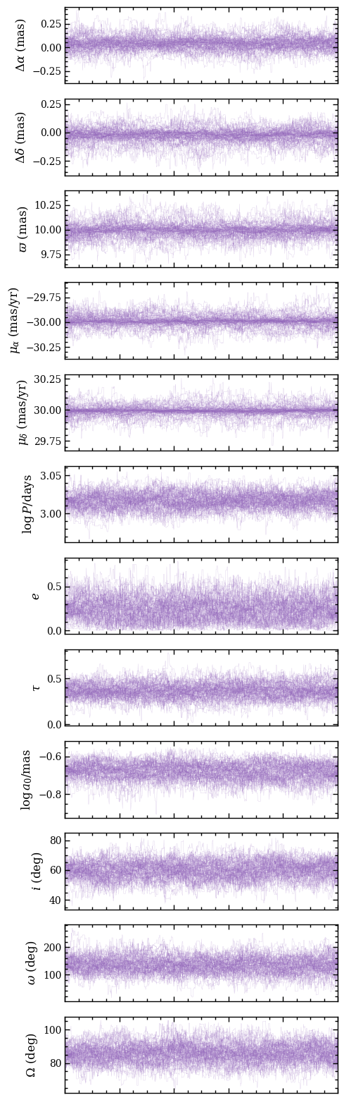
fig = results.plot_walkers(n_walkers=100, thin=None, plot_file=None)
------------
Plot walkers
------------

Number of walkers: 100
Thin value: 1
[16]:
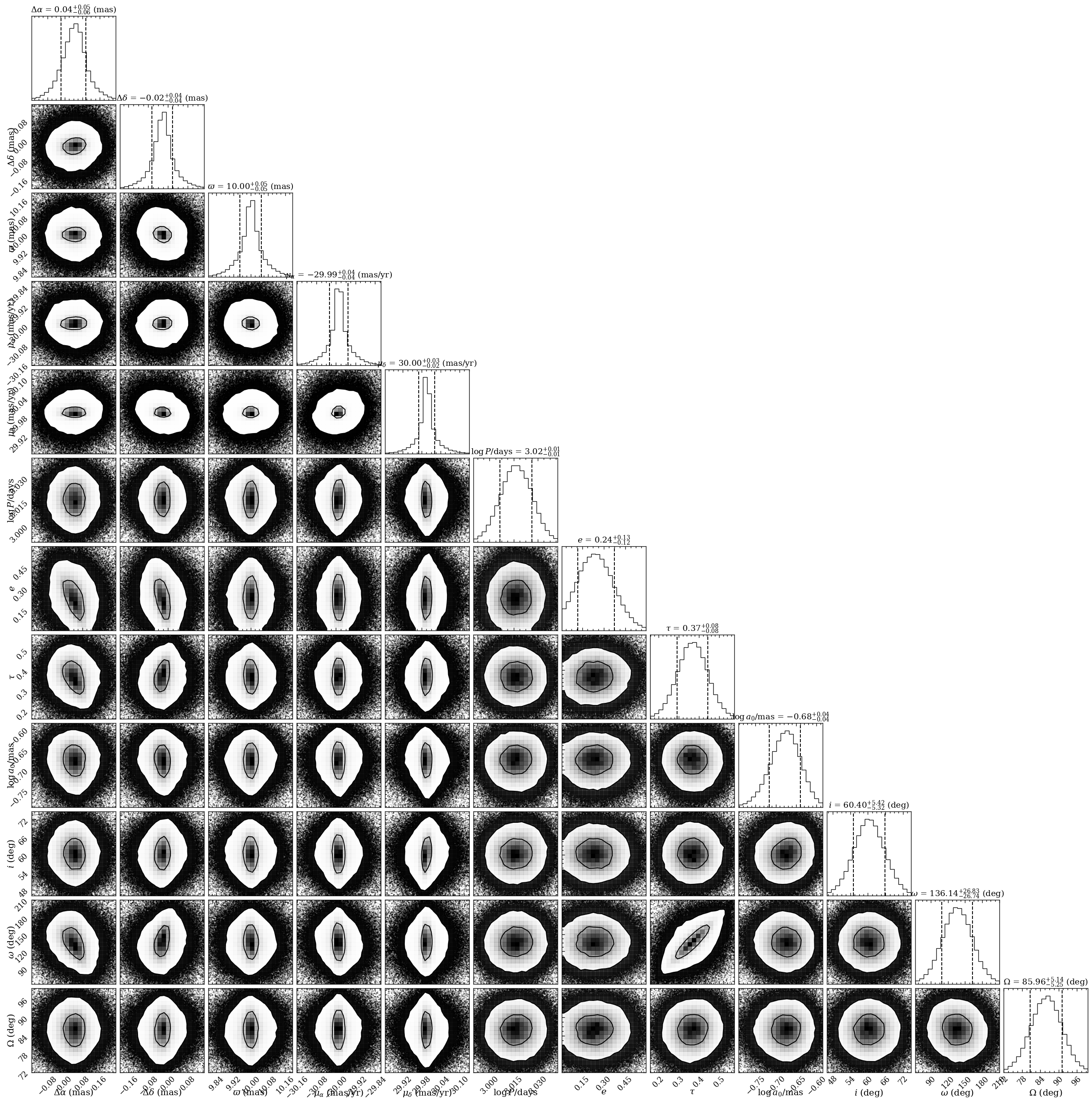
fig = results.plot_posterior(truths=None, plot_file='plot.png')
--------------
Plot posterior
--------------

Output file: plot.png
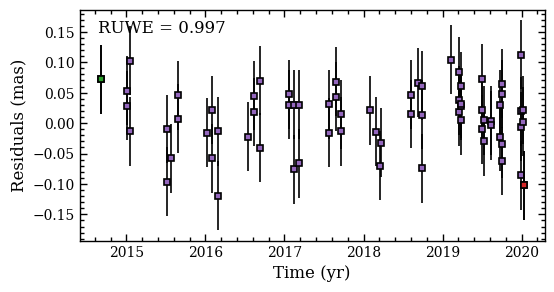
[17]:
fig = results.plot_residuals(plot_file='plot.png')
--------------
Plot residuals
--------------


-----------------------
Calculate stellar track
-----------------------

Stellar parameters:
   - RA offset (mas) = 0.058
   - Dec offset (mas) = -0.026
   - Parallax (mas) = 10.004
   - Proper motion in RA (mas/yr) = -29.992
   - Proper motion in Dec (mas/yr) = 29.994

---------------------
Calculate orbit model
---------------------

Orbit parameters:
   - Period (days) = 1031.274
   - Eccentricity = 0.194
   - Relative time of periastron = 0.307
   - Semi-major axis (mas) = 0.211
   - Inclination (deg) = 60.329
   - Argument of periastron (deg) = 118.029
   - PA of ascending node (deg) = 83.658
[18]:
fig = results.plot_orbit(plot_file='plot.png')
----------
Plot orbit
----------